Tutorial: Nonuniform Charge Density
Introduction
In this tutorial, we will explore the basic usage of μfem, focusing on several key aspects of the simulation process. Our goal is to demonstrate how to create a mesh, set up a simulation, utilize markers, define materials and boundary conditions, apply coefficient functions, and analyze simulation results through reports.
Each μfem simulation is executed through a Python script. Utilizing Python scripts offers the flexibility to customize simulations, especially when performing parameter sweeps. Furthermore, the capabilities of μfem simulations can be enhanced by integrating additional Python libraries such as NumPy, SciPy, and Matplotlib.
To run a μfem simulation defined in a Python script file (for example, case.py), you simply execute the following command in the terminal:
pymufem case.py
For those who prefer an interactive approach, you can also launch simulations by entering μfem commands directly in an IPython shell or Jupyter notebook.
Mathematical Description of the Problem
In this example, we analyze the electrostatic electric field generated by a nonuniform charge density distribution. This problem can be mathematically described using Gauss’s law, where the charge density \(\rho\) acts as the source term. In terms of the electric potential \(\phi\), the problem can be formulated as follows:
Here, we have chosen a Gaussian distribution for the charge density \(\rho\), characterized by the radius \(a\) and the peak charge \(Q\). To model this charge distribution in free space, we define the computational domain as a sphere that encircles the charge distribution. Assuming that the radius of this sphere is much larger than \(a\), we set the electric potential at its boundary \(\Gamma\) to zero. After solving this problem, we can determine the electric field using the relationship: \(\mathbf{E} = -\nabla \phi\).
To validate our results, we will compare them to an analytical solution derived from the integral form of Gauss’s law, expressed as an integral over a surface enclosing the total charge \(Q_\text{tot}\):
where \(\varepsilon_0\) is the electric permittivity of free space, \(\mathbf{E}\) is the electric field we seek, and \(d\mathbf{\Gamma}\) is a vector representing an infinitesimal area element of the surface. By choosing a sphere of arbitrary radius \(R\) as the enclosing surface, we can rewrite the equation as \(4 \pi R^2 E = Q_\text{tot} / \varepsilon_0\), which simplifies to \(E = Q_\text{tot} / 4 \pi \varepsilon_0 R^2\), where \(4 \pi R^2\) represents the surface area of the sphere. The total charge \(Q_\text{tot}\) enclosed by the sphere of radius \(R\) can be calculated using the following integral of the charge density \(\rho\):
where \(\mathrm{erf}\) is the error function.
Since the radius \(R\) of the enclosing sphere is arbitrary, we can express the electric field at any distance \(r\) as
Mesh Generation
In this section, we define the geometry of our problem and generate the corresponding mesh. For this example, we use the Gmsh mesh generator, although any software that produces a mesh in a format recognized by MFEM can be utilized (supported mesh formats).
We leverage the Gmsh Python interface for our mesh generation. First, we import the Gmsh library:
import gmsh
Next, we initialize the Gmsh API. This function must be called before any other API functions:
gmsh.initialize()
Now, we set up the geometry of our computational domain, which is represented by a sphere. We add the sphere using the OpenCASCADE CAD representation, placing it at the center (0, 0, 0) and assigning it a radius R of 10 m, which is sufficiently large to simulate free space:
R = 10.0  # [m] sphere radius

tag_domain = gmsh.model.occ.add_sphere(xc=0, yc=0, zc=0, radius=R)
The add_sphere function returns a tag, an integer that uniquely identifies the created object.
Next, we synchronize the OpenCASCADE CAD representation with the current Gmsh model:
gmsh.model.occ.synchronize()
Without this synchronization, the entities in the OpenCASCADE CAD representation will not be accessible to functions outside the OpenCASCADE CAD kernel.
We will now assign name attributes to the entities for reference in the μfem code. This will help us mark the computational domain and its boundary for applying boundary conditions. To find the boundaries of the sphere, we call the get_boundary function with the dimension and tag of the sphere:
boundary = gmsh.model.get_boundary(dimTags=[(3, tag_domain)])
tag_outer = boundary[0][1]
This function returns a list of dimension-tag pairs, and since the sphere has only one boundary, we extract the tag of the first element.
Next, we assign the name attribute “Sphere” to the sphere and “Sphere::Boundary” to its boundary using the Gmsh function add_physical_group:
gmsh.model.add_physical_group(dim=3, tags=[tag_domain], name="Sphere", tag=1)
gmsh.model.add_physical_group(dim=2, tags=[tag_outer], name="Sphere::Boundary", tag=1)
We also provide custom integer attributes using the tag keyword argument. Note that entities of different dimensions can share the same custom tags.
To generate the mesh, we set the maximum size of the mesh elements to 0.5 m and call the Gmsh mesh generation function:
gmsh.option.set_number(name="Mesh.MeshSizeMax", value=0.5)

gmsh.model.mesh.generate(dim=3)
Finally, we write the generated mesh to an external file in a format specified by the MshFileVersion option:
gmsh.option.set_number(name="Mesh.MshFileVersion", value=2.2)
gmsh.write(fileName="geometry.msh")
As a best practice, when we are done using the Gmsh API, we finalize it by calling the finalize function:
gmsh.finalize()
To summarize, here we provide the complete code to generate the mesh for our problem:
import gmsh

gmsh.initialize()

# Setup the geometry ~~~~~~~~~~~~~~~~~~~~~~~~~~~~~~~~~~~~~~~~~~~~~~~~~~~~~~~~~~~~~~~~~~~~~~
R = 10.0  # [m] sphere radius

tag_domain = gmsh.model.occ.add_sphere(xc=0, yc=0, zc=0, radius=R)

gmsh.model.occ.synchronize()

# Assign the name attributes ~~~~~~~~~~~~~~~~~~~~~~~~~~~~~~~~~~~~~~~~~~~~~~~~~~~~~~~~~~~~~~
# Define the tag of the outer boundary:
boundary = gmsh.model.get_boundary(dimTags=[(3, tag_domain)])
tag_outer = boundary[0][1]

gmsh.model.add_physical_group(dim=3, tags=[tag_domain], name="Domain", tag=1)
gmsh.model.add_physical_group(dim=2, tags=[tag_outer], name="Domain::Outer", tag=1)

# Generate the mesh ~~~~~~~~~~~~~~~~~~~~~~~~~~~~~~~~~~~~~~~~~~~~~~~~~~~~~~~~~~~~~~~~~~~~~~~
gmsh.option.set_number(name="Mesh.MeshSizeMax", value=0.5)

gmsh.model.mesh.generate(dim=3)

# Write the mesh into file:
gmsh.option.set_number(name="Mesh.MshFileVersion", value=2.2)
gmsh.write(fileName="geometry.msh")

gmsh.finalize()
Simulation Code
Setting Up the Simulation
In this section, we begin the μfem Python script by importing the μfem library. For convenience, we also import the electrostatics module under the alias estat:
import mufem
import mufem.electromagnetics.electrostatics as estat
Next, we perform the basic setup for the simulation. We create a new mufem.Simulation object, providing a custom name for the simulation (“Tutorial”) and the path to the mesh file:
sim = mufem.Simulation.New(
    name="Tutorial",
    mesh_path="source/getting_started/tutorials/nonuniform_charge_density/geometry.msh",
)
We then create an instance of the mufem.SteadyRunner class, which governs the execution of the simulation, and specify the total number of iterations (more information on simulation runners can be found in Simulation Runners). We register the runner in the simulation by calling the set_runner method:
runner = mufem.SteadyRunner(total_iterations=3)
sim.set_runner(runner)
The total number of iterations is determined empirically by observing the residual error printed by the runner at each step of the simulation. In this example the runner will output the following table:
Starting...
electromagnetics.electrostatics.ElectrostaticsModel,
1 2.657547e+05
2 9.860686e-08
3 1.712723e-11
In this table, the first number represents the iteration index, while the second indicates the residual error. We can see that three iterations are sufficient to achieve a sufficiently small residual error.
After setting up the simulation object and the runner, we configure the model for our simulations. To solve electrostatic problems, such as the one described in (1), μfem utilizes the Electrostatics Model. We create this model by calling the constructor of the ElectrostaticsModel class and passing the marker domain_marker that refers to the computational domain to which the model will be applied. We register the model in our simulation by adding it to the mufem.ModelManager:
domain_marker = "Sphere" @ mufem.Vol

model = estat.ElectrostaticsModel(marker=domain_marker, order=2)
sim.get_model_manager().add_model(model)
In this case, the domain_marker, an instance of the mufem.Marker, refers to the mesh volume with the name attribute “Sphere” that we defined during mesh generation (more information on markers can be found in Markers). To enhance simulation precision, we also pass the order=2 argument, indicating that the model should use second-order polynomial functions to approximate the solution within each finite element.
Next, we specify the type of material filling the computational domain. In our simulation, we assume that the domain is filled with air, which can be treated as having the same electric permittivity as vacuum. This material can be defined using the ElectrostaticMaterial.Constant class, which specifies an electrostatic material with constant electric permittivity, defaulting to the vacuum value. After creating the material, we register it by adding it to the model:
material = estat.ElectrostaticMaterial.Constant(name="Air", marker=domain_marker)
model.add_material(material)
We then define the Gaussian charge density distribution using the mufem.CffExpressionScalar coefficient function. This function creates a scalar coefficient from a provided mathematical expression string:
Q = 1.0  # [C] charge
a = 0.5  # [m] radius of the charge distribution
expr = f"""
    var r := sqrt(x()^2 + y()^2 + z()^2);
    var Q := {Q};
    var a := {a};

    Q / (4 * pi) * exp(-r^2 / (2 * a^2))
"""
cff_charge = mufem.CffExpressionScalar(expr)
More information on μfem coefficients can be found in Coefficients.
We use this scalar coefficient to define the source condition with an instance of the ChargeDensityCondition class:
charge_density_condition = estat.ChargeDensityCondition(
    name="Volume Charge", marker=domain_marker, charge_density=cff_charge
)
In this example, we utilize the previously created marker domain_marker to specify the region where this source condition is defined.
Following (1), we specify the boundary condition at the boundary of the computational domain. For this purpose, we use an instance of the ElectricPotentialCondition.Constant class, which allows us to set a constant electric potential of zero at the boundary:
boundary_marker = "Sphere::Boundary" @ mufem.Bnd
potential_condition = estat.ElectricPotentialCondition.Constant(
    name="Potential = 0V", marker=boundary_marker, electric_potential=0
)
To indicate the boundary of the computational domain, we use the marker that refers to the corresponding mesh entity with the name attribute “Sphere::Boundary”.
Having created the source condition and the boundary condition, we register them in the model by calling the following function:
model.add_conditions([charge_density_condition, potential_condition])
Now that the entire simulation is set up, we can run it simply by executing:
sim.run()
Analyzing the Results
After the simulation finishes, we are ready to analyze the obtained data. First, we load necessary Python libraries:
import numpy as np
import math
import matplotlib.pyplot as plt
Next, we create a function that calculates the theoretical electric field given by equation (2):
def theory(r):
    eps0 = 8.8541878188e-12  # [F/m] vacuum permittivity
    factor = Q / (4 * np.pi * eps0 * r**2)
    term1 = np.sqrt(np.pi / 2) * a**3 * math.erf(r / (np.sqrt(2) * a))
    term2 = a**2 * r * np.exp(-r**2 / (2 * a**2))
    return factor * (term1 - term2)
For simplicity, we will compare the electric field obtained from the simulations with the theoretical one only along the x-axis.To do this, we create a one-dimensional array of coordinates that spans the diameter of the sphere representing the computational domain, ranging from -R` to R` and divided into 500 points. To avoid issues when the mesh does not have an element exactly at the distance R, we add a small tolerance. Finally, we create two arrays, E_mufem and E_theory, to store the fields obtained from the simulations and those calculated using the theoretical formula:
R = 10.0  # [m] sphere radius
Nr = 500

r = np.linspace(-R + 0.01, R - 0.01, Nr)
E_mufem = np.zeros(Nr)
E_theory = np.zeros(Nr)
Next, we create a loop to iterate over all points across the diameter of the computational domain. At each step of the loop, we create a mufem.ProbeReport for a single point to access the electric field calculated by μfem (more information about reports can be found in Reports and Monitors). After evaluating this report, we extract the desired component of the electric field and store it in the E_mufem array. Similarly, we update the E_theory array by calling the previously defined theory function:
for i in range(Nr):
    report = mufem.ProbeReport.SinglePoint(
        name="Electric Field Report", cff_name="Electric Field", x=r[i], y=0, z=0,
    )
    E = report.evaluate()
    E_mufem[i] = E.x

    E_theory[i] = theory(r[i])
Finally, we plot both arrays using Matplotlib functions:
plt.figure(constrained_layout=True)
plt.plot(r, E_theory / 1e9, "k-", label="Theory")
plt.plot(r, E_mufem / 1e9, label="$\\mu$fem")
plt.legend(loc="best", frameon=False)
plt.xlabel("Distance $r$ [m]")
plt.ylabel("Electric field $E$ [GV/m]")
plt.savefig(
    "source/getting_started/tutorials/nonuniform_charge_density/images/Electric_Field.png"
)
Also, for further postprocessing and visualization, we export the electric field data into a VTK file using the field exporter (more information about the field exporter can be found in the Field Exporter):
vis = sim.get_field_exporter()
vis.add_field_output("Electric Field")
vis.save(order=2)
Here, we utilize the order=2 option in the vis.save function. This explicitly instructs the field exporter to use second-order polynomial functions to represent the field data. This choice aligns with the second-order representation used when setting up the electrostatics model, ensuring consistency in our analysis.
The Complete Code
The complete code for the example can be found below (case.py):
import mufem
import mufem.electromagnetics.electrostatics as estat

# Setup the simulation ~~~~~~~~~~~~~~~~~~~~~~~~~~~~~~~~~~~~~~~~~~~~~~~~~~~~~~~~~~~~~~~~~~~~
sim = mufem.Simulation.New(
    name="Basic Example",
    mesh_path="source/getting_started/tutorials/nonuniform_charge_density/geometry.msh",
)

runner = mufem.SteadyRunner(total_iterations=3)
sim.set_runner(runner)

# Setup the model and material ~~~~~~~~~~~~~~~~~~~~~~~~~~~~~~~~~~~~~~~~~~~~~~~~~~~~~~~~~~~~
domain_marker = "Sphere" @ mufem.Vol

model = estat.ElectrostaticsModel(marker=domain_marker, order=2)
sim.get_model_manager().add_model(model)

material = estat.ElectrostaticMaterial.Constant(name="Air", marker=domain_marker)
model.add_material(material)

# Setup the conditions ~~~~~~~~~~~~~~~~~~~~~~~~~~~~~~~~~~~~~~~~~~~~~~~~~~~~~~~~~~~~~~~~~~~~
Q = 1.0  # [C] charge
a = 0.5  # [m] radius of the charge distribution
expr = f"""
    var r := sqrt(x()^2 + y()^2 + z()^2);
    var Q := {Q};
    var a := {a};

    Q / (4 * pi) * exp(-r^2 / (2 * a^2))
"""
cff_charge = mufem.CffExpressionScalar(expr)

charge_density_condition = estat.ChargeDensityCondition(
    name="Volume Charge", marker=domain_marker, charge_density=cff_charge
)

boundary_marker = "Sphere::Boundary" @ mufem.Bnd
potential_condition = estat.ElectricPotentialCondition.Constant(
    name="Potential = 0V", marker=boundary_marker, electric_potential=0
)

model.add_conditions([charge_density_condition, potential_condition])

# Run the simulation ~~~~~~~~~~~~~~~~~~~~~~~~~~~~~~~~~~~~~~~~~~~~~~~~~~~~~~~~~~~~~~~~~~~~~~
sim.run()

# Analyze the results ~~~~~~~~~~~~~~~~~~~~~~~~~~~~~~~~~~~~~~~~~~~~~~~~~~~~~~~~~~~~~~~~~~~~~
import numpy as np
import math
import matplotlib.pyplot as plt

def theory(r):
    eps0 = 8.8541878188e-12  # [F/m] vacuum permittivity
    factor = Q / (4 * np.pi * eps0 * r**2)
    term1 = np.sqrt(np.pi / 2) * a**3 * math.erf(r / (np.sqrt(2) * a))
    term2 = a**2 * r * np.exp(-r**2 / (2 * a**2))
    return factor * (term1 - term2)

R = 10.0  # [m] sphere radius
Nr = 500

r = np.linspace(-R + 0.01, R - 0.01, Nr)
E_mufem = np.zeros(Nr)
E_theory = np.zeros(Nr)

for i in range(Nr):
    report = mufem.ProbeReport.SinglePoint(
        name="Electric Field Report", cff_name="Electric Field", x=r[i], y=0, z=0,
    )
    E = report.evaluate()
    E_mufem[i] = E.x

    E_theory[i] = theory(r[i])

plt.figure(constrained_layout=True)
plt.plot(r, E_theory / 1e9, "k-", label="Theory")
plt.plot(r, E_mufem / 1e9, label="$\\mu$fem")
plt.legend(loc="best", frameon=False)
plt.xlabel("Distance $r$ [m]")
plt.ylabel("Electric field $E$ [GV/m]")
plt.savefig(
    "source/getting_started/tutorials/nonuniform_charge_density/images/Electric_Field.png"
)

# Export the electric field data to a VTK file:
vis = sim.get_field_exporter()
vis.add_field_output("Electric Field")
vis.save(order=2)
~~~~~~~~~~~~~~~~~~~~~~~~~~~~~~~~~~~~~~~~~~~~~~~~~~~~~~~~~~~~~~~~~~~~~~~~~~~~~~

Welcome to μfem (0.2.94-dev) by Raiden Numerics LLC.


             μfem - a finite element application framework
                           __
                   _   _  / _|  ___  _ __ ___
                  | | | || |_  / _ \| '_ ` _ \
                  | |_| ||  _||  __/| | | | | |
                  |  __/ |_|   \___||_| |_| |_|
                  |_|

              https://www.raiden-numerics.com/mufem

For questions and bug reports please reach out to mufem@raiden-numerics.com
or visit https://www.raiden-numerics.com/mufem/.

Usage at own risk. No warranty provided.

License: Community (Non-commercial)

~~~~~~~~~~~~~~~~~~~~~~~~~~~~~~~~~~~~~~~~~~~~~~~~~~~~~~~~~~~~~~~~~~~~~~~~~~~~~~
Total processes: 1
Mesh: Elements(152512) Vertices(27433) Edges(186014) Faces(311094)
Starting...
electromagnetics.electrostatics.ElectrostaticsModel,
1 2.657547e+05
2 9.860686e-08
3 1.712723e-11
Simulation done. Thank you for using the software.
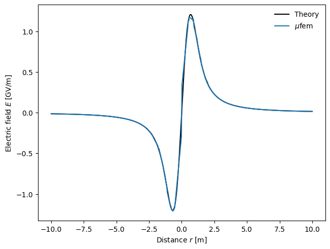
The resulting figure demonstrates that the electric field obtained from the μfem simulation closely matches the field calculated using the analytical formula.
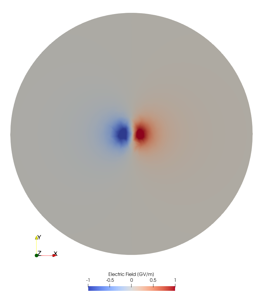
To visualize the exported electric field data, we use ParaView. The corresponding Python script is available in the paraview.py file. The following figure illustrates the distribution of the \(x\)-component of the electric field in the \(z=0\) cross-section: