Time-Domain Magnetic Model¶

Introduction¶

This model uses the quasi-static approximation of Maxwell's equations where wave and displacement effects are neglected. This model is typically used for low-frequency applications where magnetic fields and eddy currents dominate, such as electric machines, transformers, and induction heating.

The model here uses the so-called A-formulation (also known as electric formulation), where we are solving for the magnetic vector potential $\mathbf{A}$, given by:

\[ \begin{align} \operatorname{curl} \nu \operatorname{curl} \mathbf{A} + \sigma \frac{\partial \mathbf{A}}{\partial t} = \mathbf{J} + \nu \operatorname{curl} \mathbf{B}_r\, , \end{align} \]

where:

$\nu$ is the symmetric rank-2 reluctivity tensor,
$\sigma$ is the symmetric rank-2 electric conductivity tensor,
$\mathbf{J}$ is a prescribed divergence-free current density ($\operatorname{div} \mathbf{J}= 0$),
$\mathbf{B}_r$ is the remanent flux density.

Note that the magnetic flux density is related to the magnetic vector potential by:

\[ \begin{align} \mathbf{B} = \operatorname{curl} \mathbf{A}, \end{align} \]

The magnetic reluctivity is the inverse of the magnetic permeability tensor ($\nu = \mu^{-1}$). The electric conductivity tensor $\sigma$ is usually a diagonal tensor, where the off-diagonal terms are zero. It describes how well a material conducts electric current. The remanent flux density is related to the remanent magnetization ($\mathbf{M}_r$) by $\mathbf{B}_r = \mu \mathbf{M}_r$.

Equation (1) is augmented by the constitutive equations:

\[ \begin{align} \mathbf{H} &= \nu \left( \mathbf{B} - \mathbf{B}_r \right), \\ \mathbf{J} &= \sigma \mathbf{E}, \end{align} \]

Note that in general the material properties $\nu$, $\sigma$, and $\mathbf{B}_r$ can be nonlinear and dependent on other physical properties such as temperature.

In the governing equation above, the prescribed current density $\mathbf{J}$ on the right-hand side is set through support models such as the Excitation Coil Model.

Model¶

The model can be created and added to the simulation using

time_domain_magnetic_model = TimeDomainMagneticModel(
    marker=["Air", "Cylinder"] @ Vol,
    order=1,
    magnetostatic_initialization=True
)

sim.get_model_manager().add_model(time_domain_magnetic_model)

where - marker specifies the domain on which the model is solved - order is the polynomial order of the discretization - magnetostatic_initialization controls whether an initial condition is obtained by first solving the magnetostatic problem

Materials¶

The governing equation requires the provision of material properties, specifically the magnetic reluctivity (inverse permeability), the electric conductivity, and the magnetization. A material is created by specifying methods to compute each of those three material properties. Most materials can be set up using the General Material, with an example provided in Table 1.

Table 1: General Material Example
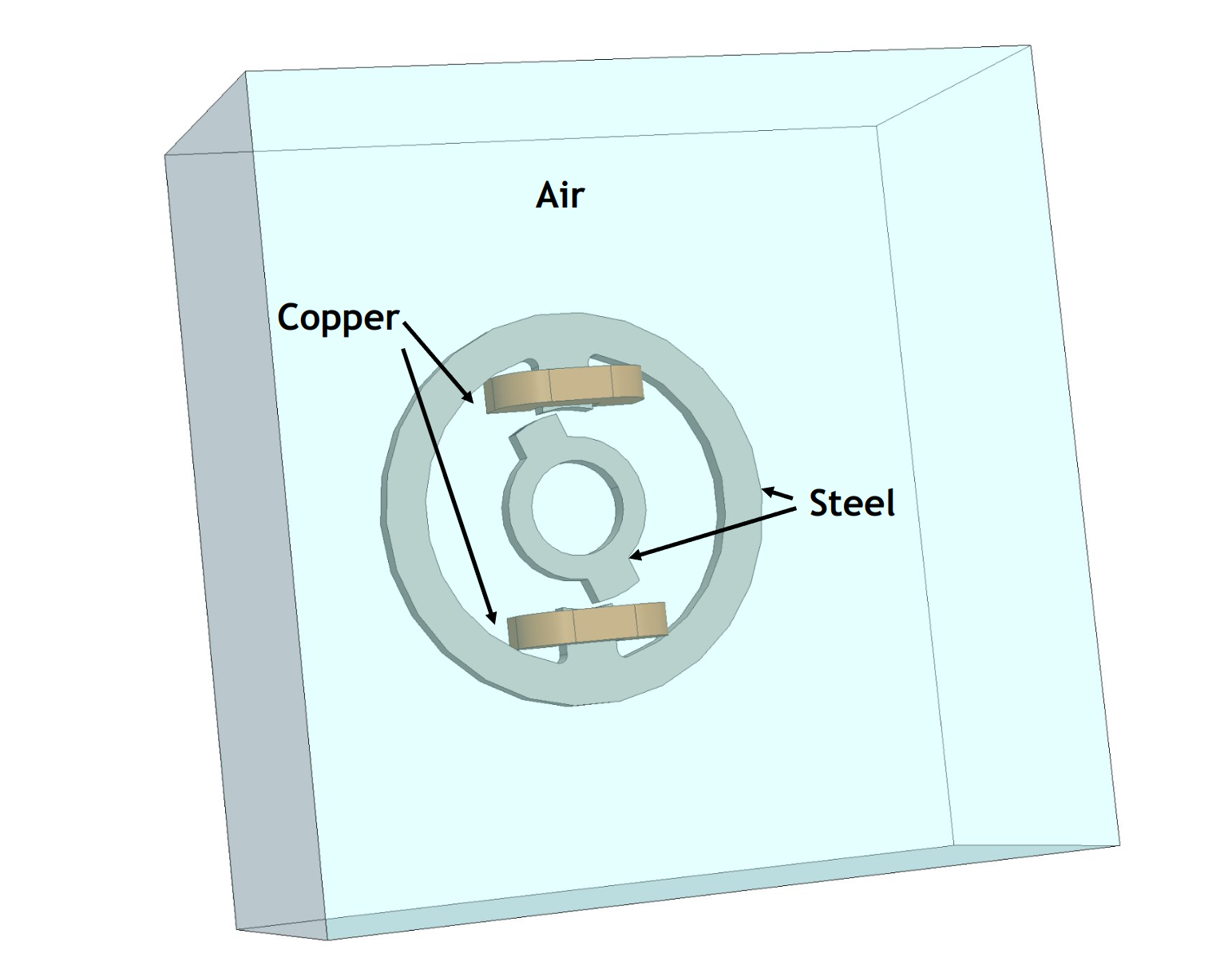Example simulation with three materials: Air, Copper and Steel.	Air For non-magnetic and non-conductive regions such as air with $$ \mu = \mu_0,\qquad \sigma = 0,\qquad \mathbf{B}_r = 0 $$ we can create the material using: `air_material = TimeDomainMagneticGeneralMaterial( name="Air", marker="Air" @ Vol )` Copper For non-magnetic but electrically conductive regions such as copper with $$ \mu = \mu_0,\qquad \sigma = \sigma_{\text{Cu}},\qquad \mathbf{B}_r = 0 $$ we can create the material using: `copper_material = TimeDomainMagneticGeneralMaterial( name="Copper", marker=["Upper Coil", "Lower Coil"] @ Vol, electric_conductivity=5.8e7, has_eddy_currents=False, )` Steel For magnetic and electrically conductive regions such as steel with $$ \mu = \mu(\|\mathbf{B}\|),\qquad \sigma = \sigma_{\text{steel}},\qquad \mathbf{B}_r = 0 $$ we can create the material using: `steel_material = TimeDomainMagneticGeneralMaterial( name="Steel", marker=["Rotor", "Stator"] @ Vol, magnetic_permeability=([0, 1000, 2000, ...], [0.0, 0.7, 1.0, ...]), electric_conductivity=4.5e6, )`

Note that, once created, the materials need to be added to the model:

time_domain_magnetic_model.add_materials([air_material, copper_material, steel_material])

More complex materials such as hysteretic, laminated, and superconducting materials are supported in their respective modules.

Conditions¶

The following conditions are available for the time-domain magnetic model:

List of supported conditions
Name	Supported Entities	Description
Tangential Magnetic Flux	Boundary	Enforces the magnetic flux density to be tangential to the boundary: $$ \mathbf{n} \cdot \mathbf{B} = 0 $$ on the boundary $\Gamma_0$.
Normal Magnetic Field	Boundary	Forces the magnetic field to be normal to the boundary by setting its tangential component to zero: $$ \left. \mathbf{H} \times \mathbf{n} \right\|_{\Gamma_0} = 0. $$
Tangential Magnetic Field	Boundary	The tangential magnetic field given by $$ \left. \mathbf{H} \times \mathbf{n} \right\|_{\Gamma_0} = \mathbf{H}_\text{usr}, $$ where $\mathbf{H}_\text{usr}$ is the user-defined external magnetic field imposed on the boundary $\Gamma_0$.

Reports¶

The following reports are available for the time-domain magnetic model:

List of reports
Name	Field Type	Description
Magnetic Force Report	Vector	Returns the total magnetic force on an object.
Magnetic Torque Report	Vector	Returns the total magnetic torque on an object.

Coefficients¶

The following functions are available for the time-domain magnetic model for visualization or querying:

List of functions
Name	Field Type	Description
Magnetic Flux Density	Vector	The magnetic flux density is computed as: $$ \mathbf{B} = \operatorname{curl} \mathbf{A}. $$
Magnetic Field	Vector	The magnetic field is given by: $$ \mathbf{H} = \nu \left( \mathbf{B} - \mathbf{B}_r \right), $$ where $\mathbf{B}_r$ is the remanent flux density.
Electric Current Density	Vector	The electric current density inside the simulation domain, which is the sum of the eddy current density and the current density from the coils.
Ohmic Heating	Scalar	The ohmic heating is computed as: $$ P_\Omega = \mathbf{J} \cdot \mathbf{E}. $$
Electric Conductivity	Symmetric Tensor	The electric conductivity tensor $\sigma$.