Time-Harmonic Magnetic Model¶

Introduction¶

The time-harmonic magnetic model describes electromagnetic fields in terms of their complex amplitudes at a single angular frequency \(\omega = 2\pi f\), under the low-frequency (eddy-current) approximation where displacement currents are neglected. This approximation is applicable when wave-propagation effects are negligible compared to diffusion/induction effects, which is typical for many low-frequency magnetic devices.

The time-harmonic magnetic model solves

\begin{align}
   \nabla \times \left( \nu \nabla \times \tilde{\mathbf{A}} \right)
   + j \omega \sigma \tilde{\mathbf{A}}
   = \tilde{\mathbf{J}}_\mathrm{s},
\end{align}

where - \(\nu = 1/\mu\) is the magnetic reluctivity - \(\sigma\) is the electric conductivity - \(\tilde{\mathbf{J}}_\mathrm{s}\) is the impressed (source) current density.

In a conductive material, the induced (eddy) current density is given by \(\tilde{\mathbf{J}} = \sigma \tilde{\mathbf{E}}\).

Model¶

The model can be created and added to the simulation using

time_harmonic_magnetic_model = TimeHarmonicMagneticModel(
    marker=magnetic_domain,
    frequency=60, 
    order=2
)

sim.get_model_manager().add_model(time_harmonic_magnetic_model)

Materials¶

In the most general case, the material parameters \(\nu\) and \(\sigma\) in Eq. (3) can be complex, frequency-dependent tensors that vary spatially and may also depend on other physical properties, such as temperature. A material is specified through the Time-Harmonic General Magnetic Material. For details refer to Time-Harmonic General Magnetic Material.

Most materials can be setup using the General Material with an example provided in Table 1.

Table 1: General Material Example

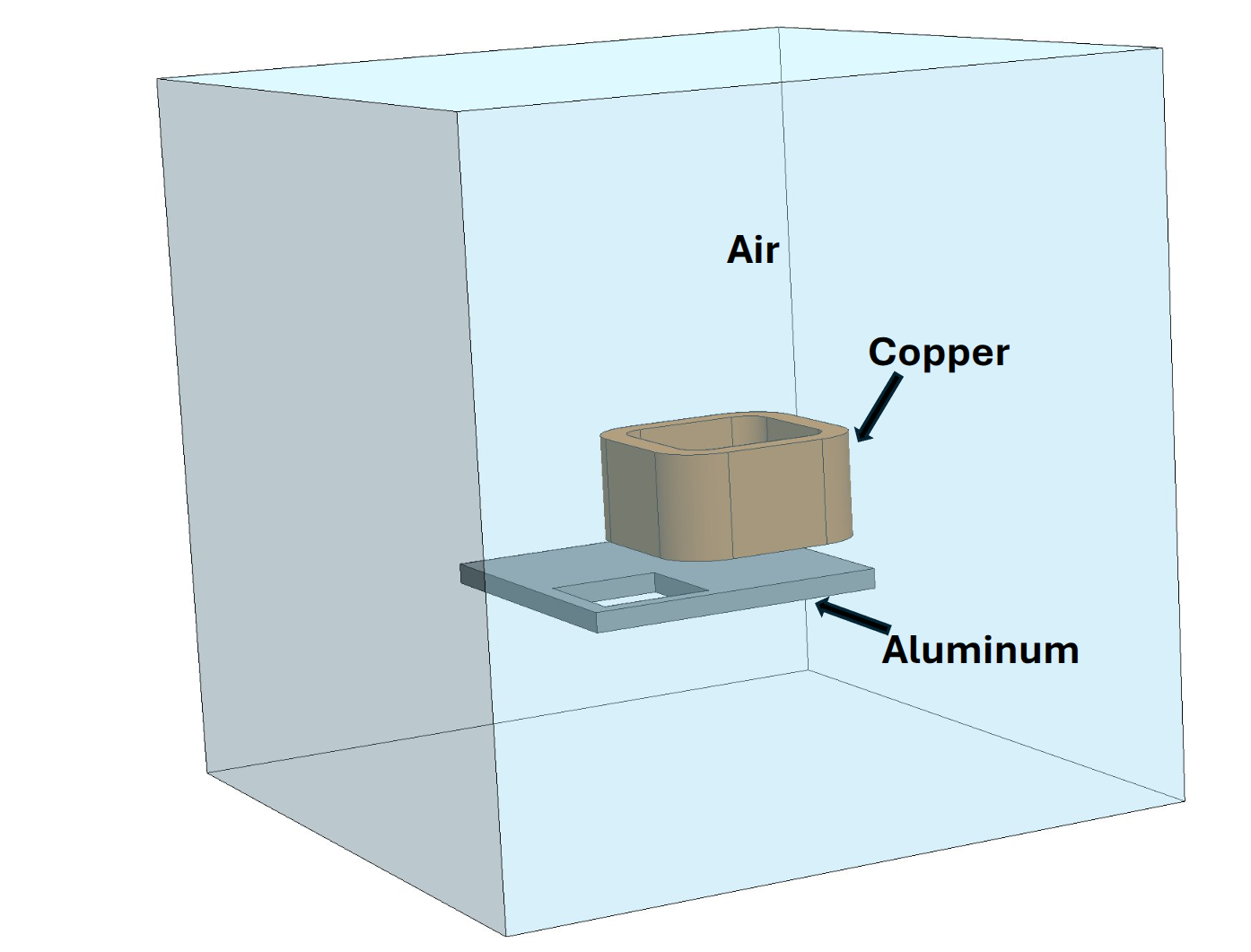Example from the Compumag TEAM-7 case. The simulation contains three materials: Air, Copper and Aluminum.

Air For non-magnetic and non-conductive regions such as air with $$ \mu = \mu_0,\qquad \sigma = 0,\qquad $$ we can create the material using: air_material = TimeDomainMagneticGeneralMaterial( name="Air", marker="Air" @ Vol ) Copper For non-magnetic but electrically conductive regions such as copper with $$ \mu = \mu_0,\qquad \sigma = \sigma_{\text{Cu}},\qquad $$ we can create the material using: copper_material = TimeDomainMagneticGeneralMaterial( name="Copper", marker=["Upper Coil", "Lower Coil"] @ Vol, electric_conductivity=5.8e7, has_eddy_currents=False, ) (note that we ignore eddy currents here due to the stranded coil). Aluminum For electrically conductive regions such as aluminum we use $$ \mu = \mu_0,\qquad \sigma = \sigma_{\text{al}},\qquad $$ we can create the material using: steel_material = TimeDomainMagneticGeneralMaterial( name="Steel", marker=["Rotor", "Stator"] @ Vol, magnetic_permeability=1.0, electric_conductivity=4.5e6, has_eddy_currents=True, )

Note that once created the materials need to be added to the model

time_harmonic_magnetic_model.add_materials([air_material, copper_material, aluminum_material])

Conditions¶

Equation (3) is solved within a specific domain and must be accompanied by appropriate boundary conditions and excitations.

Reports¶

Coefficients¶

The following functions are available in the time-harmonic magnetic model for visualization or querying: