Superconductor Material¶

⚠ Experimental feature. The superconductor material is under active development. The interface and the supported parameter ranges may change without notice.

This material models a type-II superconductor in the mixed (vortex) state, where the electric field \(\mathbf{E}\) and the current density \(\mathbf{J}\) are related by a strongly nonlinear power-law characteristic instead of ordinary Ohm's law. The power-law form is the empirical fit used in engineering practice to describe flux-creep dissipation around the critical current density. See the overview for background on the superconducting state, the critical surface and the type-I / type-II distinction.

Unlike the General Material, the superconductor material is non-magnetic (\(\mu = \mu_0\), \(\mathbf{B}_r = 0\)) but carries a strongly nonlinear, field-dependent conductivity. It must be declared with the dedicated SuperconductorMagneticMaterial class because the constitutive law is not available through the general material.

E-J power-law characteristic¶

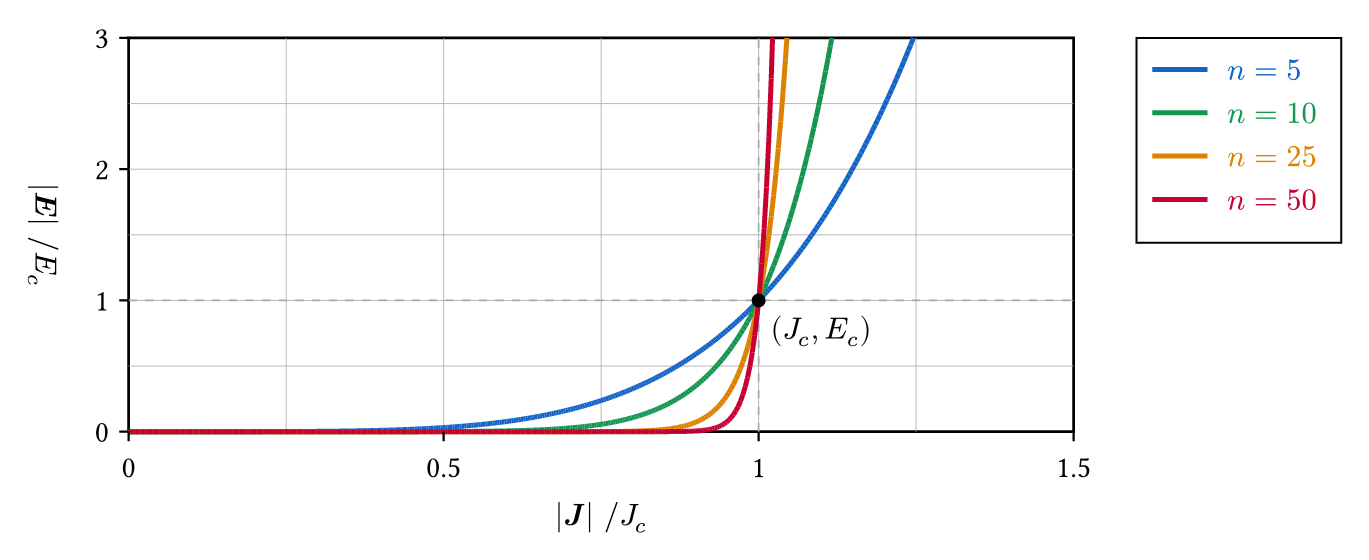
The superconductor obeys the standard E-J power law,

\[ \mathbf{E} = \frac{E_c}{J_c} \left(\frac{|\mathbf{J}|}{J_c}\right)^{n-1} \mathbf{J}\, , \]

where the three parameters

Symbol	Units	Description
\(E_c\)	V/m	Critical electric field — the characteristic field at which the sample is said to carry \(J_c\). Industry convention is \(E_c = 10^{-4}\,\mathrm{V/m}\) (\(= 1\,\mu\mathrm{V/cm}\)).
\(J_c\)	A/m²	Critical current density at the chosen \(E_c\) criterion. Sets the current-carrying capacity of the superconductor.
\(n\)	–	Power-law exponent ("n-value"). Measures the steepness of the transition between the low-loss and the flux-flow regimes. \(n \to \infty\) recovers the Bean critical-state model; \(n = 1\) recovers Ohm's law. Typical engineering range: \(n \in [20, 40]\) for commercial REBCO / Bi-2223 tapes near 77 K.

are properties of the conductor and in general depend on temperature and the local magnetic field. They are treated here as constants.

E-J power-law characteristic for different n-values

E-J power law for several n-values. All curves cross at the critical point \( (J_c, E_c) \); higher n approaches a sharp switch around \( |\mathbf{J}| = J_c \) — the curve is essentially flat for \( |\mathbf{J}| < J_c \) and rises steeply just above.

Usage¶

A superconductor material is created by specifying the marker of the conductor region and the three power-law parameters:

from mufem import Vol
from mufem.electromagnetics.module.superconductor import (
    SuperconductorMagneticMaterial,
)

hts_material = SuperconductorMagneticMaterial(
    name="Bi-2223",
    marker="Cube" @ Vol,
    Ec=1.0e-4,   # V/m — standard 1 µV/cm criterion
    Jc=2.5e6,    # A/m² — at 77 K, self-field
    n=25,        # power-law exponent for Bi-2223 at 77 K
)

time_domain_magnetic_model.add_materials([hts_material])

The material applies on the conductor region only; the surrounding air, former, or cryostat are declared with the General Material as usual.

Solver settings¶

The power-law nonlinearity is very stiff for engineering n-values (\(n \in [20, 40]\)): the constitutive curve is essentially flat below \(J_c\) and rises by orders of magnitude over a narrow band around it. A plain Picard update typically overshoots and either oscillates or diverges within the first few timesteps. We strongly recommend one of the following:

Strong under-relaxation of the nonlinear iteration, e.g.
```
magnetic_model.get_solver().set_under_relaxation_factor(0.45)
```
Values around \(0.3\) – \(0.5\) are typical; higher \(n\) asks for stronger damping. This is the simplest fix and is usually enough for AC-loss studies in the partial-penetration regime.
Line search along the Newton/Picard direction. More robust for steep transitions (large \(n\), near full penetration, or sharp transient fronts) and removes the need to hand-tune the relaxation factor at the cost of additional residual evaluations per outer iteration.

Without one of these stabilisers the outer iteration will commonly stall or blow up on superconductor regions, even when the same setup converges cleanly on normal conductors.

Reference parameters¶

Representative power-law parameters reported in the literature for commercial conductors:

Conductor	\(T\) [K]	\(E_c\) [V/m]	\(J_c\) [A/m²]	\(n\)	Notes
Bi-2223 (1G tape)	77	\(10^{-4}\)	\(\sim 2.5 \times 10^6\)	20 – 25	Bulk-equivalent \(J_c\) over tape cross-section, self-field.
REBCO (2G tape)	77	\(10^{-4}\)	\(\sim 2 \times 10^{10}\) (engineering \(J_e \sim 10^8\))	25 – 40	\(J_c\) refers to the thin REBCO layer; engineering \(J_e\) averaged over the tape is the design quantity.
NbTi	4.2	\(10^{-4}\)	\(\sim 3 \times 10^9\)	30 – 50	At 5 T, used in MRI and accelerator magnets.

These values vary strongly with temperature and applied field. Use values characterised for the operating point of the device.

References¶

K. Berger et al., Benchmark on the 3D numerical modeling of a superconducting bulk, HAL preprint hal-01548728v4 (2017). https://hal.science/hal-01548728 ↩