Newton Form
The previous pages assemble a linear system, apply constraints, and solve it. When the model is nonlinear a single solve is not enough: mufem must repeat the cycle in an outer iteration. This page describes that iteration: how mufem forms the correction, how it stabilises the step, and what the reported residual measures.
The nonlinear system
A finite-element model discretizes to a linear system \(A\,\mathbf{x} = \mathbf{b}\) (see Assembly), with system matrix \(A\), right-hand side \(\mathbf{b}\), and solution vector \(\mathbf{x}\). For a linear model \(\mathbf{x} = A^{-1}\mathbf{b}\) is exact. But in many engineering applications a material property depends on the field being solved for. Examples are a saturating \(B\)–\(H\) curve, a temperature-dependent conductivity, a radiative flux, and a power-law constitutive relation. Then the system matrix \(A(\mathbf{x})\) and possibly the right-hand side \(\mathbf{b}(\mathbf{x})\) depend on the solution itself, and
can no longer be solved in one step. Instead we define the residual vector
and adopt an iterative root-finding approach that drives \(\mathbf{r}\) toward zero. Where \(\mathbf{r}(\mathbf{x}) = \mathbf{0}\) the original system is satisfied.
| Symbol | Meaning | Depends on \(\mathbf{x}\)? |
|---|---|---|
| \(\mathbf{x}\) | Solution vector (true degrees of freedom) | – |
| \(A(\mathbf{x})\) | System (stiffness) matrix from the bilinear form; carries the material properties | yes, if a property is field-dependent |
| \(\mathbf{b}(\mathbf{x})\) | Load vector from the linear form (sources, boundary data) | only for field-dependent sources |
| \(\mathbf{r}(\mathbf{x})\) | Residual: how far \(\mathbf{x}\) is from satisfying the system | yes |
Newton's method
The iteration starts at \(n = 0\) from an initial guess \(\mathbf{x}^0\), in practice the zero vector or a value from an initial condition. It then evaluates the residual
If its norm is below the convergence threshold the solve is done. Otherwise Newton's method produces the next iterate from a first-order expansion of the residual,
where \(J(\mathbf{x}^n)\) is the Jacobian of \(\mathbf{r}\) with respect to \(\mathbf{x}\), a local linear approximation of the nonlinear residual.
The Jacobian
Differentiate \(\mathbf{r} = A(\mathbf{x})\,\mathbf{x} - \mathbf{b}(\mathbf{x})\) and use the product rule on the first term. This gives
The linear term is the ordinary system matrix. The nonlinear terms capture how \(A\) and \(\mathbf{b}\) themselves shift with the field: the differential of the reluctivity, of \(\kappa(T)\), of the power-law slope. For a linear problem the nonlinear terms vanish and the Jacobian is just the system matrix, \(J = A\).
This structure covers every source of nonlinearity. A material nonlinearity makes a property, and so \(A\), depend on the field. A geometric nonlinearity makes the operator depend on the deformed configuration, that is, again on \(\mathbf{x}\). A load nonlinearity (for example a follower load) makes \(\mathbf{b}\) depend on the field. All three enter through the same \(\partial A / \partial \mathbf{x}\) and \(\partial \mathbf{b} / \partial \mathbf{x}\) terms, so the product-rule expansion above already accounts for them.
Correction and update
With the correction vector \(\mathbf{c} = \mathbf{x}^{n+1} - \mathbf{x}^n\), equation \((1)\) becomes a linear solve for \(\mathbf{c}\),
which avoids ever forming \(J^{-1}\) explicitly. Once \(\mathbf{c}\) is known the solution is advanced,
where \(\alpha\) is a step factor, typically \(1\), damped below \(1\) by under-relaxation, or adapted (and allowed above \(1\)) by a line search, used to stabilise strongly nonlinear problems. Finally mufem recomputes the residual,
to reflect the changes in both \(A\) and \(\mathbf{b}\). It checks the norm against the convergence criterion. If the norm does not meet the criterion, a further iteration begins from equation \((1)\).
Convergence
With the full Jacobian \(J(\mathbf{x}^n)\), Newton's method converges quadratically near the solution: Newton roughly squares the error each iteration. The trade-offs are that mufem must assemble the Jacobian's nonlinear (tangent) terms, and the convergence basin is smaller. A poor initial guess or an over-large step can push the iteration away from the root. The under-relaxation factor and the line search below keep it stable and steer it toward the solution.
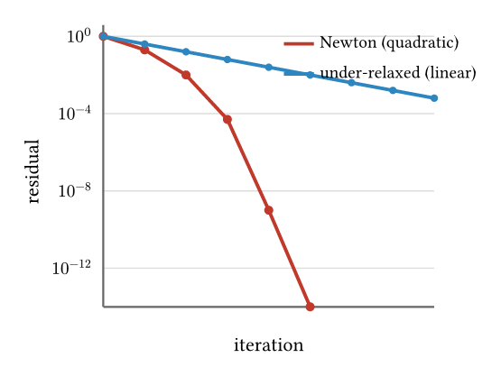
The difference in rate is dramatic. Newton roughly squares the residual each iteration once it is close, and reaches machine precision in a handful of steps. A damped or Picard iteration instead reduces the residual by a roughly constant factor, so it decays along a straight line on the logarithmic scale.
Picard fallback
A few models without a readily available tangent instead approximate the Jacobian by its linear term alone, \(J(\mathbf{x}^n) \approx A(\mathbf{x}^n)\). This Picard (successive-substitution) scheme solves the frozen-property linear system \(A(\mathbf{x}^n)\,\mathbf{c} = -\mathbf{r}^n\) each iteration. It needs no tangent but converges only linearly rather than quadratically.
Under-relaxation
The simplest way to tame an unstable iteration is to apply only a fixed fraction of the correction:
A value \(\alpha < 1\) damps each update. This slows convergence (more iterations) but prevents the overshoot that occurs when the linearization is only locally valid. This overshoot is the typical failure mode of strongly nonlinear materials: the full step lands far from the true solution and the iteration oscillates or stalls. Examples are deeply saturated magnetic cores, radiative boundary terms, and steep power-law constitutive relations. Under-relaxation is the standard first remedy when a residual refuses to fall.
The factor is set per model on its solver and stays constant for the whole run:
The default is 1.0 (no damping). Every implicit solver exposes this control.
Line search
A fixed under-relaxation factor is a compromise: too large near the solution (wastefully conservative once the iteration is well-behaved) and possibly still too large far from it. A line search removes the guesswork by choosing \(\alpha\) automatically at every outer iteration, small when the step is risky, up to and beyond \(1\) when it is safe.
Rather than the correction norm, the line search looks at how the problem's objective changes along the correction direction. It treats the directional derivative
as a function of the step length and picks the \(\alpha\) that drives \(g\) to zero (a stationary point of the objective along the ray). Because \(g\) is smooth, mufem finds this root cheaply by extrapolation from a couple of trial evaluations ("probes") of the step, then clamps the result to a safe range so a single bad fit cannot take a wild step. A final backtrack halves \(\alpha\) if the residual \(\lVert \mathbf{r} \rVert\) actually grew after the step, guaranteeing the accepted step never makes things worse.
Three extrapolation strategies are available, trading accuracy for cost:
| Strategy | Description |
|---|---|
TwoPointLinear | Two probes (\(\alpha = 0.5\) and \(1.0\)), linear fit of \(g(\alpha)\), one root. The cheapest option and the default. |
ThreePointQuadratic | Adds a third, cost-free anchor \(g(0)\) recovered from the just-solved linear system and fits a quadratic, captures one more order of nonlinearity at the same probe cost. |
ResidualMinimization | Fits \(\lVert \mathbf{b}(\alpha) \rVert^2\) directly and minimises it. Prefer this when the objective-stationary and residual-minimal steps diverge, i.e. stiff constitutive laws that settle at a stationary point with non-zero residual (e.g. the \(\rho\)-floor regime in high-temperature superconductors). |
The line search is currently offered by the Time-Domain Magnetic model and is inactive by default. When inactive, the solver applies the configured under-relaxation factor. Access it through the solver:
solver = magnetic_model.get_solver()

line_search = solver.get_line_search()
line_search.set_active(True)
line_search.set_strategy(mufem.LineSearchStrategy.ThreePointQuadratic)

# Forbid over-relaxation (α never exceeds 1) for stiff power-law materials
line_search.set_max_alpha(1.0)
| Method | Description |
|---|---|
set_active(active) | Turn the line search on or off. Default off. |
set_strategy(strategy) | Select the extrapolation strategy (see table). Default TwoPointLinear. |
set_max_alpha(max_alpha) | Upper clamp on the accepted \(\alpha\). Default 2.0; set to 1.0 to forbid over-relaxation. The lower clamp is fixed at 0.05. |
set_iteration_window(min_iter, max_iter) | Restrict the line search to outer iterations in the given (1-indexed, inclusive) range. |
set_residual_skip_threshold(threshold) | Skip the line search while \(\lVert \mathbf{r} \rVert\) is below this value, falling back to the under-relaxation factor. Default 0 (never skip). |
Under-relaxation vs. line search
The two are complementary, not exclusive. The under-relaxation factor is the step applied whenever the line search is off, outside its iteration window, or when its fit degenerates, so it acts as the safe fallback. Enabling the line search lets mufem adapt around that fallback instead of holding a single conservative value for the whole run.
The reported residual
A natural convergence measure is the \(L_2\) norm of the residual vector, \(\lVert \mathbf{r} \rVert_2 = \sqrt{\mathbf{r}\cdot\mathbf{r}}\). mufem does not report this directly. The correction solves \(J\,\mathbf{c} = -\mathbf{r}\) with a non-singular \(J\), so the correction \(\mathbf{c}\) vanishes exactly when \(\mathbf{r}\) does. So the size of the correction is an equivalent convergence signal, and mufem monitors it. Concretely, the value printed in the Residual column is the relative Euclidean norm of the correction against the updated iterate:
| Symbol | Meaning |
|---|---|
| \(\mathbf{c}\) | Correction vector for this iteration (before under-relaxation) |
| \(\lVert \cdot \rVert_2\) | Euclidean (\(\ell_2\)) norm over all true degrees of freedom, summed across MPI ranks |
| \(\varepsilon\) | Machine-safe floor preventing division by zero when the iterate is exactly zero (e.g. the first step from a zero guess) |
This ratio is dimensionless and mesh-independent by construction: numerator and denominator scale together under refinement, so a single tolerance works across problems of different physical scale and resolution. Two details worth knowing:
- The raw correction \(\mathbf{c}\) is used in the numerator, not the under-relaxed step \(\alpha\,\mathbf{c}\). This is deliberate: with \(\alpha = 0\) the solution would not move, yet \(\mathbf{c}\) can still be large, scaling by \(\alpha\) would falsely report convergence.
- For complex fields (time-harmonic models) the real and imaginary parts contribute to the norms: \(\lVert \mathbf{c} \rVert_2^2 = \lVert \mathbf{c}_{\mathrm{re}} \rVert_2^2 + \lVert \mathbf{c}_{\mathrm{im}} \rVert_2^2\).
A converged solve drives \(r_{\mathrm c}^{\,n}\) toward zero. For a purely linear model it reaches round-off after a single iteration.
Reading the output
The residual of every model that reports one is printed after each iteration as a table. Each column corresponds to one model. The value is \(r_{\mathrm c}^{\,n}\) in scientific notation. mufem reprints the header every 25 iterations.
Iteration |   Time-Domain Magnetic |
        1 |           1.254886e+00 |
        2 |           4.258440e-01 |
        3 |           7.038054e-02 |
        4 |           8.631071e-03 |
        5 |           4.057884e-03 |
A model that is frozen
(held fixed while other physics advance) shows Frozen instead of a number.
Healthy convergence looks like a residual that falls by several orders of magnitude and then plateaus near round-off. A residual that stalls at a large value, oscillates, or grows indicates the outer iteration is not converging. To fix it, add under-relaxation, increase the iteration budget, or check the material model.
Querying residuals in Python
The recorded residuals are also available from the Model Manager at runtime.
model_manager = sim.get_model_manager()

# All reporting models, keyed by display name: {"Time-Domain Magnetic": [r0, r1, ...]}
history = model_manager.get_residuals()

# The residual sequence of one model, addressed by its class name
residuals = model_manager.get_model_residuals("electromagnetic.TimeDomainMagneticModel")
| Method | Description |
|---|---|
get_residuals() | Dictionary mapping each reporting model's display name (the column shown in the table) to its list of residuals. |
get_model_residuals(model_name) | Residual sequence for a single model, keyed by its class name (e.g. electromagnetic.TimeDomainMagneticModel). Entries are None for iterations in which the model was frozen. |
Controlling convergence
The outer loop runs for the number of iterations configured on the
runner (SteadyRunner(total_iterations=...), or the inner
iterations of an UnsteadyRunner). The residual is a diagnostic: mufem does
not stop the loop automatically, so the iteration count should be chosen large
enough for the residual to settle, and the printed table used to confirm it did.
Each model's solver exposes the knobs that shape convergence, the under-relaxation factor, the line search (where available), the linear-solver tolerances, and the linear-solver iteration cap. See the individual Solver pages, for example the Time-Harmonic Magnetic Solver, for the exact defaults and setters.