Overview
mufem is built on the finite element method (FEM), the standard numerical approach for solving the partial differential equations (PDEs) of physics on realistic geometry. FEM does not seek a closed-form solution. It divides the domain into a mesh of small, simple elements (triangles, tetrahedra, and so on) and approximates the unknown field by low-order polynomials on each element. You require the governing equation to hold in an averaged (weak) sense over this approximation. This converts the continuous problem into a large but sparse system of linear algebraic equations that a computer can solve.
The appeal of the method is its generality: it handles curved boundaries, spatially varying material properties, and mixed boundary conditions naturally. Its accuracy improves systematically as you refine the mesh or raise the polynomial order. mufem represents each physical field in the finite-element space that best suits it, which is why it uses nodal, edge, and other element families across its models.
The starting point is the mesh. A discrete domain \(\Omega_h\) made of elements approximates the continuous domain \(\Omega\), which is bounded by \(\Gamma\). The discrete domain has a corresponding boundary \(\Gamma_h\).
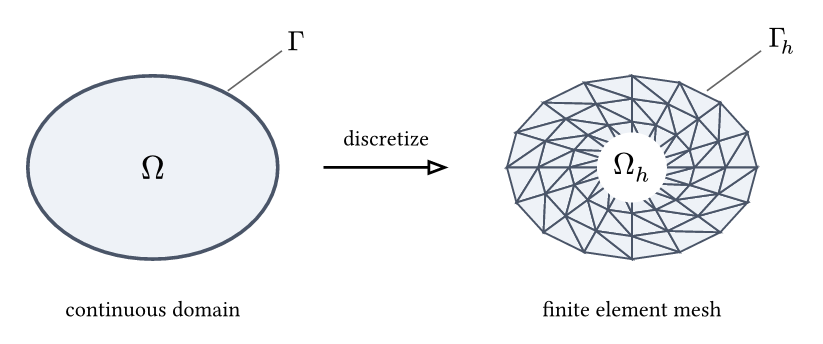
This section explains how the method turns a physical model into a system of equations, and how mufem solves that system. The pages follow the solution pipeline from left to right.

| Stage | What it does |
|---|---|
| Weak Form | Recast the governing partial differential equation in variational form, and separate essential from natural boundary conditions. |
| Discretization | Replace the continuous field with a finite-element space, turning the weak form into the linear system \(A\,\mathbf{x} = \mathbf{b}\). |
| Assembly | Build \(A\) and \(\mathbf{b}\) from element matrices computed by numerical integration. |
| Constraints | Impose Dirichlet values and multi-point ties (hanging nodes, periodicity) on the assembled system. |
| Linear Solvers | Solve \(A\,\mathbf{x} = \mathbf{b}\) with a direct or a preconditioned iterative method. |
For a linear, stationary model this pipeline runs once. Two situations wrap it in an outer iteration that re-assembles and re-solves:
- Newton Form: when the model is nonlinear, the assemble-solve cycle repeats until the residual is small.
- Time Stepping: for a transient model, the cycle repeats once per time step.
A related page covers Mesh Refinement, which adapts the finite-element space itself between solves.