Solid Temperature Model¶

Introduction¶

The solid temperature model describes how temperature changes in a solid. It uses thermal conduction with internal heat sources. It also supports heat exchange at the solid boundaries through convection and radiation. The governing transient heat equation is $$ \begin{align} \rho c_p \frac{\partial T}{\partial t} - \nabla \cdot (\kappa \nabla T) = Q. \end{align} $$

$T$ - temperature [K]
$\rho$ - material density [kg/m$^3$]
$c_p$ - specific heat capacity [J/(kg K)]
$\kappa$ - thermal conductivity [W/(m K)]
$Q$ - volumetric heat power density [W/m$^3$]

You typically use the model for:

Thermal-management studies in electric machines and transformers.
Induction-heating workpieces.
Electronics cooling.
Welding and casting simulations.
Any solid-conduction problem with convective, radiative, or prescribed-flux boundaries.

Model¶

You create the model and add it to the simulation with

solid_thermal_model = SolidTemperatureModel(
    marker=["Plate"] @ Vol,
    order=1,
)

sim.get_model_manager().add_model(solid_thermal_model)

where - marker specifies the domain on which the model is solved - order is the polynomial order of the discretization

Materials¶

In general, the material parameters $\rho$, $c_p$, and $\kappa$ in the governing equation can vary in space. They can also be direction-dependent or depend on other physical quantities. You can define these dependencies with material functions. You give them as analytical expressions, tabulated data, or numerical models. Details are provided in Solid Temperature Material.

Table 1: General Material Example
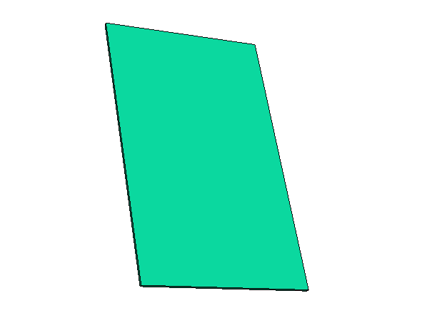Example of a silicon plate.	Silicon The silicon plate has the following properties: $$ \begin{alignat}{2} \kappa &= 111 \quad &\left[ \mathrm{W} / (\mathrm{m} \cdot \mathrm{K}) \right] \\ c_p &= 668 &\left[ \mathrm{J} / (\mathrm{kg} \cdot \mathrm{K}) \right] \\ \rho &= 2330 &\left[ \mathrm{kg} / \mathrm{m}^3 \right] \end{alignat} $$ We can create the material using: `silicon_material = SolidTemperatureMaterial( name="Silicon", marker="Plate" @ Vol, thermal_conductivity=111.0, specific_heat_capacity=668.0, density=2330.0, )`

After you create the materials, add them to the model:

solid_thermal_model.add_material(silicon_material)

Conditions¶

List of supported conditions
Name	Supported Entities	Description
Adiabatic	Boundary	Enforces zero normal heat flux (perfect thermal insulation, no heat transfer).
Convection	Boundary	Models heat exchange with a surrounding fluid using Newton’s cooling law.
Heat Flux	Boundary	Prescribes the normal heat flux across the boundary (including zero-flux case).
Radiation	Boundary	Models radiative heat transfer between the surface and its surroundings.
Temperature	Volume, Boundary	Prescribes a fixed temperature within a volume or on a boundary (Dirichlet condition).
Volumetric Heat Source	Volume	Defines internal heat generation within the material domain.
Mushy Zone	Volume	Linear latent-heat storage term over a solidus / liquidus temperature range — phase-change problems (casting, welding, thermal storage).
Matching Interface	Boundary pair	Stitches the temperature DOFs of two geometrically coincident boundaries on separately-meshed bodies, giving a continuous temperature across the interface.

Coefficients¶

The following functions are available in the solid temperature model for visualization or querying:

List of functions
Name	Field Type	Description
Temperature	Scalar	Temperature: $T$ [K]
Density	Scalar	Material density: $\rho$ [kg/m$^3$]
Specific Heat Capacity	Scalar	Specific heat capacity: $c_p$ [J/(kg K)]
Thermal Conductivity	Scalar	Thermal conductivity: $\kappa$ [W/(m K)]

Solver¶

The model exposes a solver instance that configures convergence and damping.

You get and configure the solver with

solver = model.get_solver()
solver.set_verbose(True)
solver.set_under_relaxation_factor(0.7)

See Solver for more details.