Assembly
From weak form to a linear system
Each model in mufem states its physics as a weak (variational) form on the computational mesh. Assembly is the step that turns that continuous form into a finite system of algebraic equations for the degrees of freedom \(\mathbf{x}\):
| Symbol | Meaning |
|---|---|
| \(\mathbf{x}\) | Solution vector, the coefficients of the discretized field (the true degrees of freedom) |
| \(A\) | System (stiffness) matrix, assembled from the bilinear part of the weak form; its entries carry the material properties |
| \(\mathbf{b}\) | Right-hand side (load vector), assembled from the linear part: sources and boundary data |
Element matrices
The unknown field is expanded in the basis functions of a finite-element space. On each mesh element \(e\) the weak form reduces to a small dense element matrix \(A_e\) and element vector \(\mathbf{b}_e\). A stiffness entry is an integral over the element of products of the basis functions (or their gradients), weighted by the local material property \(\kappa\):
| Symbol | Meaning |
|---|---|
| \(\Omega_e\) | The element domain |
| \(\phi_i\) | Basis (shape) function of local degree of freedom \(i\) |
| \(\kappa\) | Material property from the weak form (conductivity, reluctivity, ...) |
The reference element
To integrate over an arbitrary physical element \(\Omega_e\), mufem pulls it back to a single fixed reference element \(\hat\Omega\) (for example the unit triangle). The basis functions and the quadrature points are defined once on this reference element. A mapping that runs in both directions relates the two elements. The parametrization \(\mathbf{x}(\boldsymbol{\xi})\) sends the reference element to the physical one. It is built from the element's geometry nodes, whose geometry order sets how curved it can be. Its inverse \(\boldsymbol{\xi}(\mathbf{x})\) maps the physical element back to the reference.
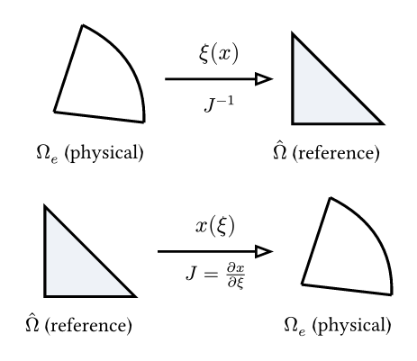
The derivative of the parametrization is the Jacobian matrix
which encodes how the reference coordinates stretch and rotate into physical coordinates. Two quantities derived from it appear in every element integral:
- its determinant \(|J|\), the local volume-scaling factor that converts the reference measure to the physical one, \(\mathrm{d}\Omega = |J|\, \mathrm{d}\hat\Omega\);
- its inverse transpose \(J^{-\mathsf{T}}\), which maps reference-space gradients to physical ones, \(\nabla_{\mathbf{x}}\phi = J^{-\mathsf{T}}\, \nabla_{\boldsymbol{\xi}}\hat\phi\).
Because mufem pulls everything back to the reference element, it tabulates the basis functions and quadrature rule once and reuses them for every element. Only \(J\) and \(|J|\), evaluated from each element's geometry, change. For a straight-sided (affine) element \(J\) is constant. For a curved element it varies from point to point.
Numerical integration
You almost never evaluate these integrals in closed form. Instead a quadrature rule samples the integrand at a fixed set of points \(\boldsymbol{\xi}_q\) inside the element and forms a weighted sum:
where \(w_q\) are the quadrature weights and \(|J|\) is the Jacobian determinant introduced above, evaluated at each quadrature point. mufem uses Gauss quadrature, whose rule of order \(m\) integrates polynomials up to degree \(m\) exactly. A higher order uses more quadrature points, as shown here on a tetrahedron:
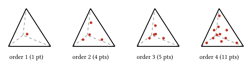
mufem chooses the order so it captures the integrand accurately. The order grows with:
- the element order \(p\): higher-order basis functions raise the polynomial degree of the integrand;
- curved elements, where the Jacobian \(|J|\) varies across the element;
- field-dependent properties, where \(\kappa\) is not constant over the element.
Too low an order under-integrates the system and can destabilise the solution. Too high an order costs more. For an order-\(p\) element with a constant property, a rule exact to degree \(2p\) is a typical default.
Scattering into the global system
Assembly then scatters the element contributions into the global system:
where \(P_e\) is the local-to-global map that sends each element degree of freedom to its global index. mufem then adds the entries of \(A_e\) into the rows and columns of \(A\) at those global indices. A degree of freedom shared by several elements accumulates a contribution from each. The figure below shows one element, whose three local nodes carry global indices \(\{2, 5, 7\}\). It scatters its \(3 \times 3\) matrix into those rows and columns of the global matrix.
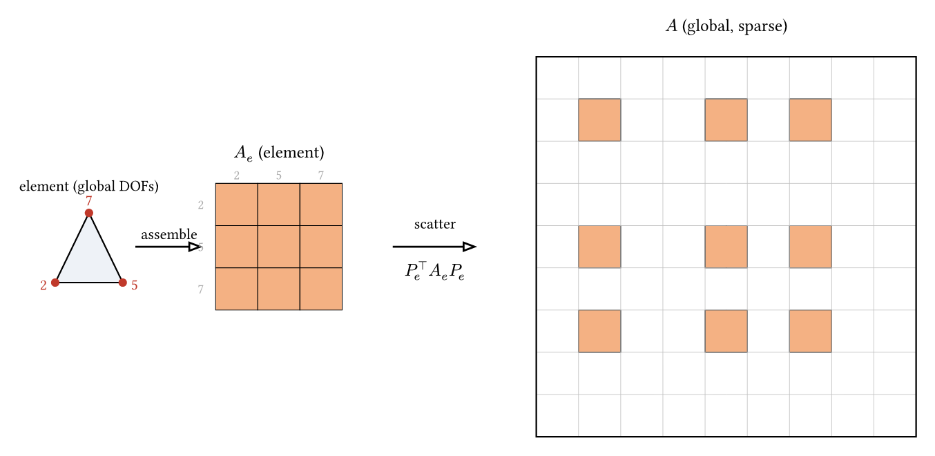
Because each element couples only the few degrees of freedom it contains, the assembled matrix \(A\) is large and sparse: most entries are zero, and only the non-zeros are stored.
Before the solver receives this system, mufem imposes the boundary and coupling constraints on \(A\) and \(\mathbf{b}\).