Discretization
Finite-element spaces
The weak form is posed over an infinite-dimensional function space \(V\). Discretization replaces that continuous space with a finite-dimensional finite-element space \(V_h \subset V\) built on the mesh. This space is a set of basis functions (also called shape functions) \(\phi_i\). Each basis function is a low-order polynomial supported on a handful of neighbouring elements and associated with one degree of freedom.
Any field in the space is a weighted sum of these basis functions,
so the unknown becomes the finite vector of coefficients \(\mathbf{x} = (x_j)\), the true degrees of freedom.
By default the scalar basis is the nodal Lagrange family. Each function is interpolatory: it equals one at its own node and zero at every other node. The nodes sit at Gauss–Lobatto points for stability at high order. The vector-valued spaces use the Nédélec and Raviart–Thomas families instead, listed below.
Solution order
The solution order (or polynomial order) \(p\) is the degree of the basis
polynomials on each element. It is chosen per model, through the order argument
of a model constructor. Order 1 uses linear basis functions with degrees of
freedom only at the element vertices. Higher orders add degrees of freedom on the
edges (and faces, and interior) and can represent curved variation of the field
within a single element. The one-dimensional nodal Lagrange basis functions look
like this:
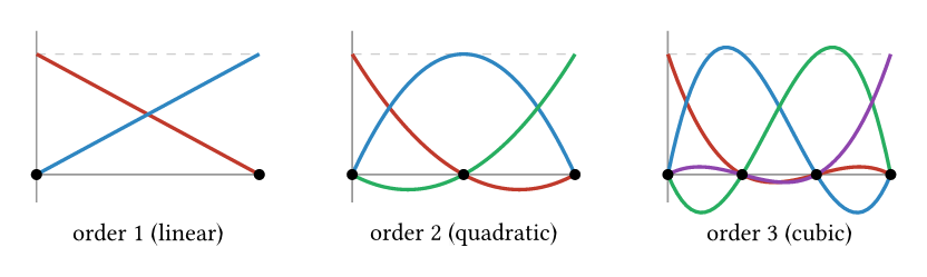
Each basis function is one at its own node and zero at all the others, so the coefficient \(x_j\) is the field value at node \(j\). Raising the order resolves smooth fields more accurately for a given mesh (p-refinement), at the cost of more degrees of freedom per element. It is the same order that adaptive refinement can raise locally.
Geometry order
The order of the solution and the order of the geometry are independent. The geometry order is the polynomial degree used to map each reference element to its actual shape in the mesh. At order 1 the elements are straight-sided (affine). At order 2 and above the edges and faces can curve to follow the true domain boundary, which matters for curved geometry such as fillets, bores, and circular arcs. The figure shows a single element edge approximating a circular boundary as the geometry order increases:
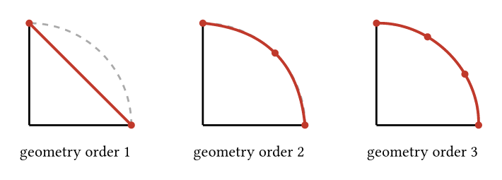
A straight edge (order 1) cuts across the curve. A quadratic (order 2) or cubic (order 3) edge follows it far more closely, with extra high-order nodes placed on the true boundary. When the geometry order equals the solution order the element is called isoparametric. mufem uses the geometry order stored in the mesh, so it represents a mesh with curved (high-order) elements using curved element edges.
Choose the two orders together. A geometry order lower than the solution order gives a subparametric element, for example a third-order solution on straight-sided first-order elements. The mesh then cannot follow a curved boundary any better than its low-order shape allows. On a domain with curved boundaries the geometry error caps the overall accuracy. Near those boundaries the element loses the fast convergence the high-order solution would otherwise deliver. A geometry order that matches the solution order removes that bottleneck. On a polygonal domain, where straight-sided elements are already exact, first-order geometry with a high solution order is perfectly fine.
The Galerkin system
Galerkin's method uses the same space for the trial field \(u_h\) and the test functions. Substitute \(u_h = \sum_j x_j \phi_j\) into the weak form \(a(u_h, v) = \ell(v)\) and test against each basis function \(v = \phi_i\) in turn. This gives one equation per degree of freedom:
with
These integrals are evaluated element by element during assembly. Because each basis function overlaps only its neighbours, most \(A_{ij}\) vanish and \(A\) is sparse.
Conforming spaces
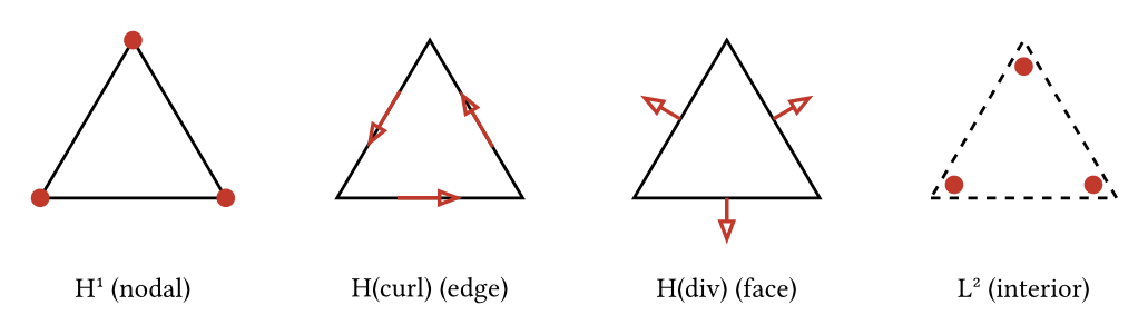
The basis must reproduce the continuity that the physics needs across element boundaries. mufem uses the standard family of conforming spaces, choosing the one that matches each field. They differ in where the degrees of freedom live on each element, sketched below for a triangle:
| Space | Continuity / degrees of freedom | Typical fields |
|---|---|---|
| \(H^1\) (nodal / Lagrange) | Fully continuous; nodal values | Temperature, electric potential, displacement, scalar potentials |
| \(H(\mathrm{curl})\) (Nédélec edge) | Tangential component continuous; edge circulations | The magnetic vector potential in electromagnetics |
| \(H(\mathrm{div})\) (Raviart–Thomas) | Normal component continuous; face fluxes | Flux-type vector fields |
| \(L^2\) (discontinuous) | No continuity imposed | Auxiliary and piecewise quantities |
Matching the space to the field is not a detail. Tangentially-continuous edge elements represent the magnetic vector potential correctly, where a nodal basis would not. This choice is also why electromagnetic solves need the specialised auxiliary-space preconditioner noted in Linear Solvers.
Discontinuous Galerkin
Not every formulation builds continuity into the space. A Discontinuous Galerkin (DG) method uses a fully discontinuous \(L^2\) basis: each element carries its own independent degrees of freedom and the field may jump across element faces. Numerical flux terms on the interior faces then restore the inter-element coupling weakly, rather than the basis itself.
This trades more degrees of freedom for element-local operators and a natural treatment of discontinuities. mufem uses a DG formulation for Maxwell problems, where the numerical flux couples neighbouring elements across each shared face.