Materials Overview¶

The time-domain magnetic model solves the magnetic vector potential ($\mathbf{A}$) form of the eddy-current equation,

\[ \underbrace{\nabla \times \left(\mu^{-1}\,\nabla \times \mathbf{A}\right)}_{\text{magnetic response}} \;+\; \underbrace{\sigma\,\frac{\partial \mathbf{A}}{\partial t}}_{\text{eddy currents}} \;=\; \mathbf{J}_s \;+\; \underbrace{\nabla \times \left(\mu^{-1}\,\mathbf{B}_r\right)}_{\text{permanent magnetization}}, \]

where $\mathbf{J}_s$ is a prescribed source current density. Each material region is characterized by three properties — one per labelled term:

The magnetic permeability $\mu$ — how strongly the material magnetizes in response to an applied magnetic field. For a linear medium it sets the constitutive relation $\mathbf{B} = \mu \mathbf{H}$.
The electrical conductivity $\sigma$ — how readily the material carries free charges. Under a time-varying magnetic field it governs the induced eddy currents and the associated Joule losses.
The remanent flux density $\mathbf{B}_r$ — the magnetization the material retains in the absence of any external field. This is what models permanent magnets.

In general these parameters can be nonlinear, anisotropic, and depend on external state such as temperature. In practice most engineering problems can be treated with an isotropic and linear $\sigma$ and $\mathbf{B}_r$; the permeability is the main source of nonlinearity (saturation in ferromagnets) and of anisotropy (laminations, single-crystal materials).

Property methods for $\mu$, $\sigma$, and $\mathbf{B}_r$ — and how to combine them into a usable material — are described on the General Material page.

Materials whose behavior falls outside this picture are covered by dedicated modules: superconductors, laminated stacks, thermal plasmas, hysteretic materials, and irreversible magnets.

Magnetic Classification¶

From a modeling perspective, materials are commonly grouped according to how they respond to an applied magnetic field:

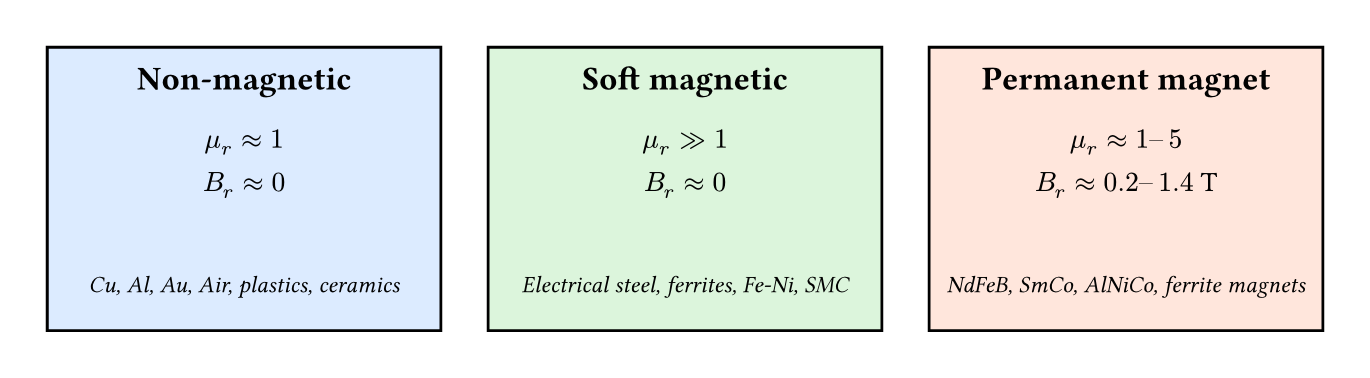Magnetic material classification Materials are commonly grouped into three engineering categories based on their permeability and remanence.

Non-magnetic materials — $\mu_r \approx 1$, $\mathbf{B}_r \approx 0$.
Soft magnetic materials — $\mu_r \gg 1$, $\mathbf{B}_r \approx 0$.
Permanent magnet materials — $\mu_r \approx 1\text{–}5$, large $\mathbf{B}_r$. Also known as hard magnetic materials.

The relative permeability $\mu_r$ is defined relative to the vacuum permeability through $\mu = \mu_r \mu_0$.

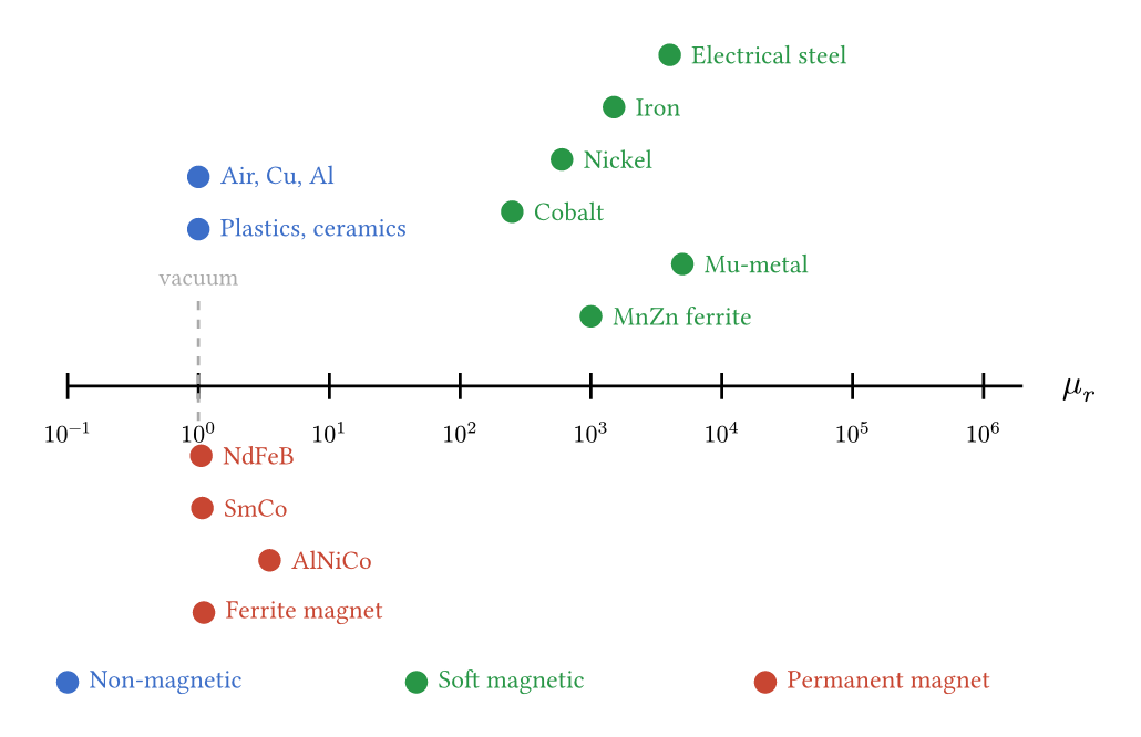Relative permeability of common materials Order of magnitude of the relative permeability for typical engineering materials, on a logarithmic scale. Non-magnetic materials cluster around $\mu_r \approx 1$, soft magnetic materials span several decades, and hard magnets remain close to unity despite carrying a large remanent flux density.

Non-Magnetic Materials¶

Non-magnetic materials have a permeability very close to that of vacuum ($\mu \approx \mu_0$) and exhibit negligible magnetization when exposed to a magnetic field.

The deviation from vacuum is captured by the magnetic susceptibility $\chi_r = \mu_r - 1$. By sign convention,

diamagnetic materials have $\chi_r < 0$,
paramagnetic materials have $\chi_r > 0$,

but in both cases $|\chi_r|$ is of order $10^{-5}$ or smaller.

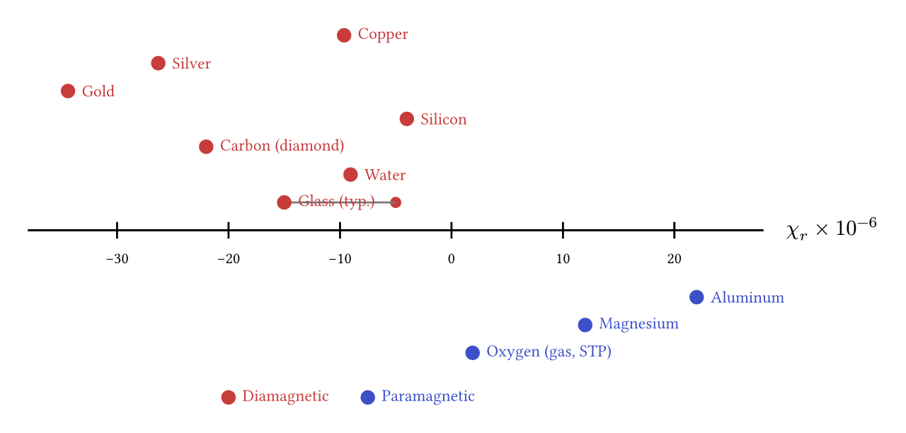Susceptibility of common non-magnetic materials Susceptibility $\chi_r$ of common non-magnetic materials. The deviation from vacuum permeability is so small that it is usually negligible in finite-element simulations.

In practice it is safe to use the vacuum permeability for these materials as the deviation is overshadowed by discretization error. They are best configured with the non-magnetic permeability method on the General Material.

Soft Magnetic Materials¶

Soft magnetic materials are easily magnetized and demagnetized and are used to guide and concentrate magnetic flux. They have high permeability and follow the applied field closely. A small residual magnetization remains after the field is removed, but it is usually negligible and not modeled here (hysteretic materials have their own dedicated module).

Typical examples include electrical steels, ferrites (MnZn, NiZn), iron-based alloys, metallic glasses, and soft-magnetic composites.

Engineering role:

Guide and concentrate magnetic flux.
Used in components where the magnetic field varies in time.
Core materials for transformers, inductors, and motor stators.

In simplified modeling they are represented by a nonlinear permeability $\mu(B)$; losses and hysteresis are typically ignored in first-order analyses.

The permeability comes from alignment of microscopic magnetic moments with the applied field. The alignment is proportional to the field at low amplitudes, but saturates once most moments are aligned. This saturation is described by the B–H curve:

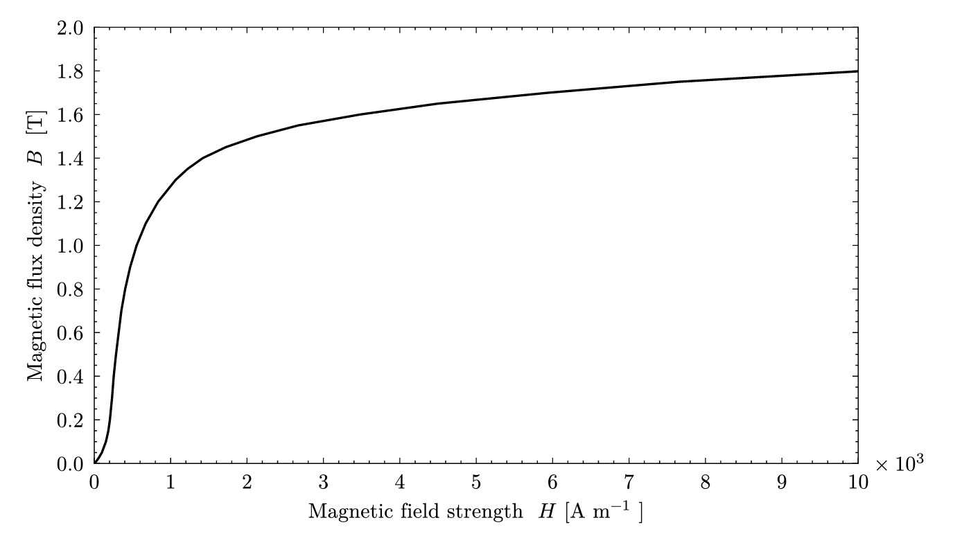Full BH curve of a soft magnetic material Full B–H curve. One usually distinguishes the initial Rayleigh region, the quasi-linear region, the transition region, and the saturation region.

Permanent Magnet Materials¶

Permanent magnet materials — also known as hard magnetic materials — are designed to retain magnetization and act as sources of magnetic field. They carry a large remanent flux density $\mathbf{B}_r$ together with a high resistance to demagnetization.

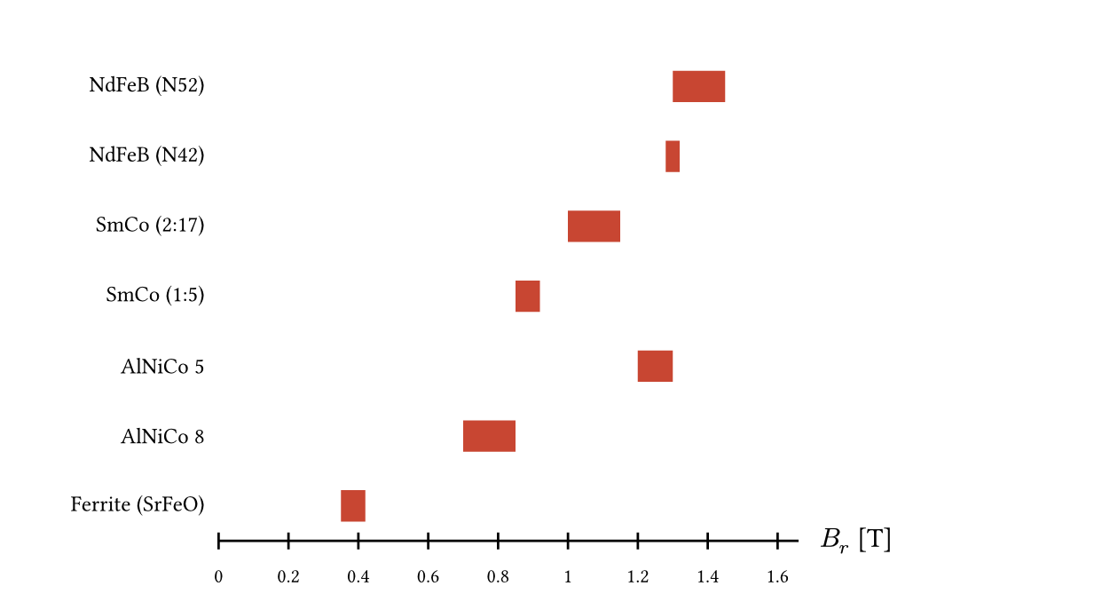Remanent flux density of common permanent magnets Range of the remanent flux density $B_r$ for the main families of permanent-magnet materials at room temperature.

Typical examples: NdFeB, SmCo, AlNiCo, ferrite magnets.

Engineering role:

Act as sources of magnetic field where a persistent field is required.
Common in permanent-magnet motors, sensors, and actuators.

In simplified modeling they are treated as regions with an imposed magnetization (or equivalent source term); their permeability is approximated as constant and close to $\mu_0$.

Electric Classification¶

The electrical conductivity varies by many orders of magnitude across materials and is conveniently grouped into three categories:

Insulators ($\sigma \lesssim 1$ S/m) — plastics, ceramics, dry gases, distilled water, intrinsic silicon. No appreciable eddy currents on practical time scales.
Lossy media ($\sigma \approx 1\text{–}10^{5}$ S/m) — everything between insulators and metals: electrolytes (sea water, brine, body fluids, molten salts) and conducting non-metals (graphite, ferrites).
Metals ($\sigma \gtrsim 10^{5}$ S/m) — copper, aluminum, iron, and other metals.

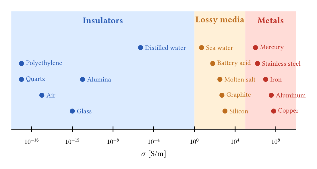Electrical conductivity of common materials on a logarithmic scale, spanning more than thirty decades. Real values often span a range that depends on temperature, composition, and humidity.

Conducting media carry both impressed currents and eddy currents induced by a time-varying magnetic field. In the time-domain magnetic model, every region is therefore classified as conducting or non-conducting depending on whether eddy currents are resolved — this is controlled by the has_eddy_currents flag on the General Material. For materials with low conductivity or laminated cores, it is generally recommended to suppress eddy currents and capture losses through other means.